Introduction

Urban Greenspace and Asthma Prevalence

This project examines the link between vegetation cover (using average NDVI as a measurement of vegetation health) and human health. In this notebook, I will calculate patch, edge, and fragmentation statistics for urban greenspace in Washington, D.C. These statistics reflect the connectivity and distribution of urban greenspace, which are important for ecosystem function and accessibility. I then use a linear model to identify statistically significant correlations between greenspace distribution and health data compiled by the U.S. Centers for Disease Control and Prevention (CDC).

Using ‘Big Data’ in the Form of Census Tracts

For this project, I divide the greenspace (NDVI) data by census tract to align with the CDC’s human health data. Because I need detailed information on the structure of greenspace within each tract, I require high-resolution data. Therefore, I use National Agricultural Imagery Program (NAIP) data, which is collected for the continental U.S. every few years at 1-meter resolution. While NAIP data is primarily intended for agricultural purposes, it is also an excellent resource for analyzing urban environments, where small-scale changes can have significant impacts.

References

City-Data. (n.d.a). Income in Denver, Colorado. City-Data.com. Retrieved March 18, 2025, from https://www.city-data.com/income/income-Denver-Colorado.html

City-Data. (n.d.b). Diversity in Denver, Colorado. City-Data.com. Retrieved March 18, 2025, from https://www.city-data.com/city/Denver-Colorado.html#mapOSM?mapOSM[zl]=11&mapOSM[c1]=39.762626183293456&mapOSM[c2]=-104.85694885253908&mapOSM[s]=sql1&mapOSM[fs]=false.

Centers for Disease Control and Prevention. PLACES: Local Data for Better Health. Atlanta, GA: U.S. Department of Health and Human Services, Centers for Disease Control and Prevention, 2023. Available at https://www.cdc.gov/places.

Set Up Analysis

Import Libraries

import pandas as pd
import rioxarray as rxr # Work with geospatial raster data
import geopandas as gpd
import pathlib
import os
import hvplot.pandas
import geoviews as gv
import cartopy.crs as ccrs
gv.extension('bokeh')  # Activates GeoViews with the Bokeh backend

# For the NDVI Data
import re # Extract metadata from file names
import zipfile # Work with zip files
from io import BytesIO # Stream binary (zip) files
import numpy as np # Unpack bit-wise Fmask
import requests # Request data over HTTP
import pystac_client
import rioxarray.merge as rxrmerge
import shapely
import xarray as xr
import glob
from cartopy import crs as ccrs
from scipy.ndimage import convolve
from sklearn.model_selection import KFold
from scipy.ndimage import label
from sklearn.linear_model import LinearRegression
from sklearn.model_selection import train_test_split
from tqdm.notebook import tqdm

warnings.simplefilter('ignore')

# Prevent GDAL from quitting due to momentary disruptions
os.environ["GDAL_HTTP_MAX_RETRY"] = "5"
os.environ["GDAL_HTTP_RETRY_DELAY"] = "1"

STEP 2: Create a Site Map

Use the Center for Disease Control (CDC) Places dataset for human health data to compare with vegetation. CDC Places also provides some modified census tracts, clipped to the city boundary, to go along with the health data. Start by downloading the matching geographic data, and then select the City of Denver, Colorado.

# Define info for CDC download, and only download cdc data once
if not os.path.exists(cdc_data_path):
    cdc_data_url = ('https://data.cdc.gov/download/x7zy-2xmx/application%2Fzip')
    cdc_data_gdf = gpd.read_file(cdc_data_url)
    denver_gdf = cdc_data_gdf[cdc_data_gdf.PlaceName=='Denver']
    denver_gdf.to_file(cdc_data_path, index=False)

# Load in cdc data
denver_gdf = gpd.read_file(cdc_data_path)

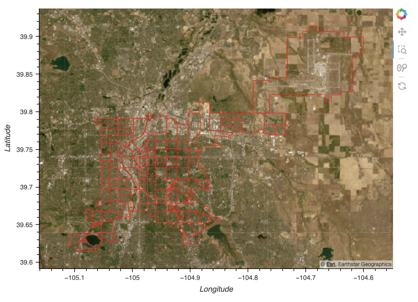
# Check the data - site plot 
denver_gdf.plot()

(
    denver_gdf
    .to_crs(ccrs.Mercator())
    .hvplot(
        line_color='red', fill_color=None,
        crs=ccrs.Mercator(), tiles='EsriImagery',
        frame_width=600
    )
)

Census Tracts in Denver, Colorado

City of Denver Data Description

Data is drawn from the Center for Disease Control PLACES: Local Data for Better Health data set. The Places Dataset estimates chronic disease and other health-related measures at various geographic levels of the United States using a small area estimation methodology. Data are derived from Behavioral Risk Factors Surveillance System data, Census population data, and American Community Survey data. There are a total of 40 measures genereated in the 2024 release.

For this analysis, I will be using data from the city level - specifically the city of Denver.

For information on how to access this data via the CDC portal, you can follow this tutorial.

You can obtain urls for the U.S. Census Tract shapefiles from the TIGER service. You’ll notice that these URLs use the state FIPS, which you can get by looking it up (e.g. here, or by installing and using the us package.

# Define info for big data download (Colorado)
census_data_co_url=("https://www2.census.gov/geo/tiger/TIGER2024/PLACE/tl_2024_08_place.zip"
)

census_data_co_dir = os.path.join(data_dir, 'census_data_co')
os.makedirs(census_data_co_dir, exist_ok=True)
census_data_co_path = os.path.join(census_data_co_dir, 'tl_2024_08_place.shp') # Spatial Join 

# Only download the census tracts once
if not os.path.exists(census_data_co_path):
    census_data_co_gdf = gpd.read_file(census_data_co_url)
    census_data_co_gdf.to_file(census_data_co_path)
    den_census_gdf = census_data_co_gdf[census_data_co_gdf.NAME=='Denver']
    den_census_gdf.to_file(census_data_co_gdf, index=False)
    

# Load in census tract data
census_data_co_gdf = gpd.read_file(census_data_co_path)

Step 3 - Access Asthma and Urban Greenspaces Data

# Set up a path for the asthma data
cdc_path = os.path.join(data_dir, 'asthma.csv')

# Download asthma data (only once)
if not os.path.exists(cdc_path):
    asthma_url = (
        "https://data.cdc.gov/resource/cwsq-ngmh.csv"
        "?year=2022"
        "&stateabbr=CO"
        "&countyname=Denver"
        "&measureid=CASTHMA"
        "&$limit=1500"
    )
    asthma_df = (
        pd.read_csv(asthma_url)
        .rename(columns={
            'data_value': 'asthma',
            'low_confidence_limit': 'asthma_ci_low',
            'high_confidence_limit': 'asthma_ci_high',
            'locationname': 'tract'})
        [[
            'year', 'tract', 
            'asthma', 'asthma_ci_low', 'asthma_ci_high', 'data_value_unit',
            'totalpopulation', 'totalpop18plus'
        ]]
    )
    asthma_df.to_csv(asthma_path, index=False)

# Load in asthma data
asthma_df = pd.read_csv(asthma_path)

# Preview asthma data
asthma_df

Join Health Data with Census Tract Boundaries

# Join the census tract GeoDataFrame with the asthma prevalence DataFrame using the .merge() method.
# Note: You will need to change the data type of one of the merge columns to match, e.g. using .astype('int64')

# Change tract identifier datatype for mergingusing the .merge()method
denver_gdf.tract2010 = denver_gdf.tract2010.astype('int64')

# Merge census data with geometry
merged_gdf = (
    denver_gdf
    .merge(asthma_df, left_on='tract2010', right_on='tract', how='inner')
)

# Plot asthma data as chloropleth
(
    gv.tile_sources.EsriImagery
    * 
    gv.Polygons(
        merged_gdf.to_crs(ccrs.Mercator()),
        vdims=['asthma', 'tract2010'],
        crs=ccrs.Mercator()
    ).opts(color='asthma', colorbar=True, tools=['hover'])
).opts(width=600, height=600, xaxis=None, yaxis=None)

Asthma Prevalence in Denver, Colorado

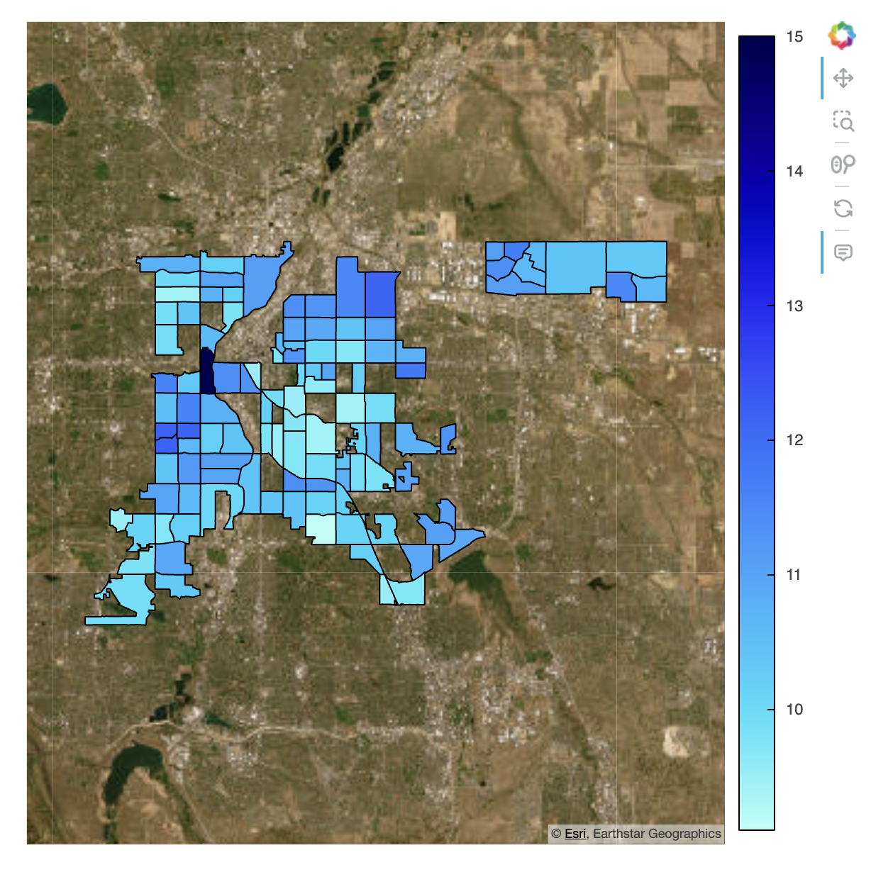
Interpretation

There appears to be a mild geographical correlation with the distribution of adults who have asthma. However, it is unclear whether this is a direct relationship or a byproduct of another variable. Other potential contributing factors include income disparity, high pollution levels due to heavy industry, or limited access to affordable healthcare. I explore these possibilities further later in this project.

Connect to the planetary computer catalog

e84_catalog = pystac_client.Client.open(
    "https://planetarycomputer.microsoft.com/api/stac/v1"
)
e84_catalog.title

# Use a loop and for each Census track search for the approrpiate data. 
# Convert geometry to lat/lon for STAC
merged_latlon_gdf = merged_gdf.to_crs(4326)

# Define a path to save NDVI stats
ndvi_stats_path = os.path.join(data_dir, 'denver-ndvi-stats.csv')

# Check for existing data - do not access duplicate tracts
downloaded_tracts = []
if os.path.exists(ndvi_stats_path):
    ndvi_stats_df = pd.read_csv(ndvi_stats_path)
    downloaded_tracts = ndvi_stats_df.tract.values
else:
    print('No census tracts downloaded so far')
    
# Loop through each census tract
scene_dfs = []
for i, tract_values in tqdm(merged_latlon_gdf.iterrows()):
    tract = tract_values.tract2010
    # Check if statistics are already downloaded for this tract
    if not (tract in downloaded_tracts):
        # Retry up to 5 times in case of a momentary disruption
        i = 0
        retry_limit = 5
        while i < retry_limit:
            # Try accessing the STAC
            try:
                # Search for tiles
                naip_search = e84_catalog.search(
                    collections=["naip"],
                    intersects=shapely.to_geojson(tract_values.geometry),
                    datetime="2021"
                )
                
                # Build dataframe with tracts and tile urls
                scene_dfs.append(pd.DataFrame(dict(
                    tract=tract,
                    date=[pd.to_datetime(scene.datetime).date() 
                          for scene in naip_search.items()],
                    rgbir_href=[scene.assets['image'].href for scene in naip_search.items()],
                )))
                
                break
            # Try again in case of an APIError
            except pystac_client.exceptions.APIError:
                print(
                    f'Could not connect with STAC server. '
                    f'Retrying tract {tract}...')
                time.sleep(2)
                i += 1
                continue

Join Dataframes Together

# Concatenate the url dataframes
if scene_dfs:
    scene_df = pd.concat(scene_dfs).reset_index(drop=True)
else:
    scene_df = None

# Preview the URL DataFrame
scene_df

Calculate the NDVI, Mask, and Determine Edge Density

# Skip this step if data are already downloaded 
if not scene_df is None:
    ndvi_dfs = []
    # Loop through the census tracts with URLs
    for tract, tract_date_gdf in tqdm(scene_df.groupby('tract')):
        # Open all images for tract
        tile_das = []
        for _, href_s in tract_date_gdf.iterrows():
            # Open vsi connection to data
            tile_da = rxr.open_rasterio(
                href_s.rgbir_href, masked=True).squeeze()
            
            # Clip data
            boundary = (
                merged_gdf
                .set_index('tract2010')
                .loc[[tract]]
                .to_crs(tile_da.rio.crs)
                .geometry
            )
            crop_da = tile_da.rio.clip_box(
                *boundary.envelope.total_bounds,
                auto_expand=True)
            clip_da = crop_da.rio.clip(boundary, all_touched=True)
                
            # Compute NDVI
            ndvi_da = (
                (clip_da.sel(band=4) - clip_da.sel(band=1)) 
                / (clip_da.sel(band=4) + clip_da.sel(band=1))
            )

            # Accumulate result
            tile_das.append(ndvi_da)

               # Merge data
        scene_da = rxrmerge.merge_arrays(tile_das)

        # Mask vegetation
        veg_mask = (scene_da>.3)

        # Calculate statistics and save data to file
        total_pixels = scene_da.notnull().sum()
        veg_pixels = veg_mask.sum()

        # Calculate mean patch size
        labeled_patches, num_patches = label(veg_mask)
        
        # Count patch pixels, ignoring background at patch 0
        patch_sizes = np.bincount(labeled_patches.ravel())[1:] 
        mean_patch_size = patch_sizes.mean()

        # Calculate edge density
        kernel = np.array([
            [1, 1, 1], 
            [1, -8, 1], 
            [1, 1, 1]])
        edges = convolve(veg_mask, kernel, mode='constant')
        edge_density = np.sum(edges != 0) / veg_mask.size
        
        # Add a row to the statistics file for this tract
        pd.DataFrame(dict(
            tract=[tract],
            total_pixels=[int(total_pixels)],
            frac_veg=[float(veg_pixels/total_pixels)],
            mean_patch_size=[mean_patch_size],
            edge_density=[edge_density]
        )).to_csv(
            ndvi_stats_path, 
            mode='a', 
            index=False, 
            header=(not os.path.exists(ndvi_stats_path))
        )

# Re-load results from file
ndvi_stats_df = pd.read_csv(ndvi_stats_path)
ndvi_stats_df

Plot the Data

# Merge census data with geometry
merged_ndvi_gdf = (
    merged_gdf
    .merge(
        ndvi_stats_df,
        left_on='tract2010', right_on='tract', how='inner')
)

# Plot choropleths with vegetation statistics
def plot_chloropleth(gdf, colorbar_opts=None, **opts):
    """Generate a choropleth with the given color column and colorbar label"""
    return gv.Polygons(
        gdf.to_crs(ccrs.Mercator()),
        crs=ccrs.Mercator()
    ).opts(
        xaxis=None, 
        yaxis=None, 
        colorbar=True,
        colorbar_opts=colorbar_opts,   
        xlabel="Longitude",
        ylabel="Latitude",
        **opts 
    )

# Generate plots with correct colorbar labels
(
    plot_chloropleth(
        merged_ndvi_gdf, 
        color='asthma', 
        cmap='viridis', 
        title="Asthma Rates by Census Tract", 
        colorbar_opts={'title': "Asthma Rate"}  # Fixed here
    ) 
    +
    plot_chloropleth(
        merged_ndvi_gdf, 
        color='edge_density', 
        cmap='Greens',
        title="Vegetation Density by Census Tract in Denver", 
        colorbar_opts={'title': "Edge Density"}  # Fixed here
    )
)

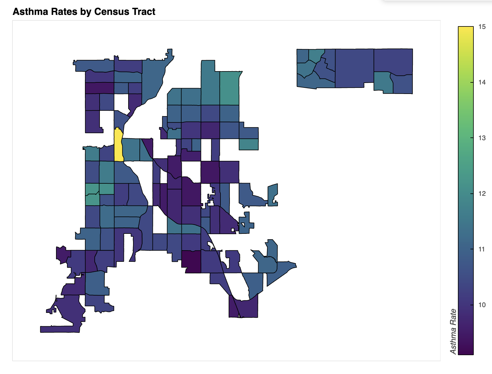
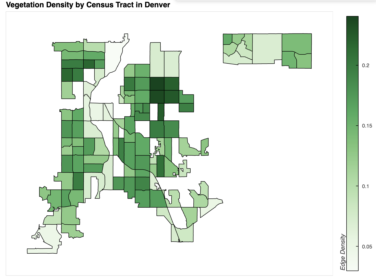
Plot Description and Comparison

Several correlations emerge between the two plots and other data sources, suggesting a slight link between vegetation density and asthma rates. However, stronger correlations have been found between asthma and factors such as income, ethnicity, and proximity to highways or industrial areas.

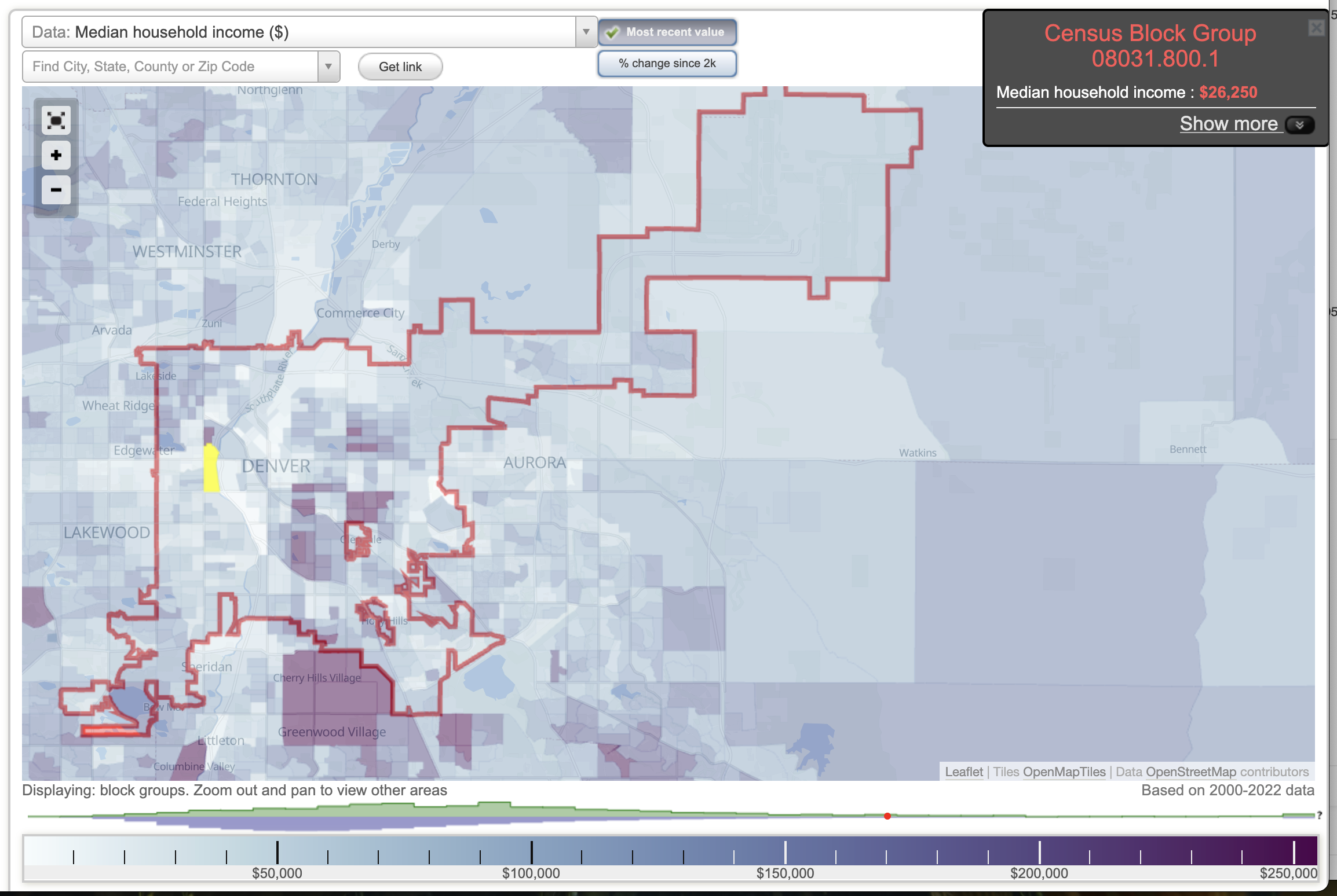
In the income map of Denver, lower-income areas generally align with higher asthma rates. For example, the census tract highlighted in the Asthma Incidence map has an average income of approximately $26,000, whereas the area directly to the north—where asthma rates are significantly lower—has a median income of $240,000 (City-Data.com, n.d.a.).

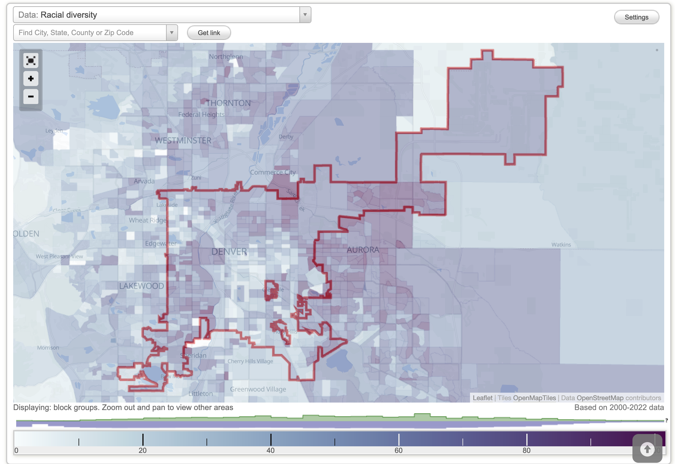
Another map that closely matches asthma prevalence is one depicting racial and ethnic diversity. Communities with the lowest diversity also tend to have the lowest asthma rates (City-Data.com, n.d.b.).

Denver Median Income

Diversity Density in Denver, CO