Understanding Animal Behavior Post Fire
During 2020, Colorado and Wyoming experienced three mega-fires, the Camron Peak, East Troublsome, and Mullen Fires, which burned over 230,000 ha. In 2024 and 2025 researchers from Colorado State University (Dr Leah McTigue) and the USDA (Dr Zack Steel) sampled 134 burned and unburned locations across a gradient of burn severity.
Objective
Bat specific - Understanding the effects of fire on bats is critical for developing effective management guidelines and policies to prevent further endangerment and foster recovery.
General - Determine the response post-fire across species and assess chanages in occupancy and biodiversity across pyrodiversity and elevation change. The goal is to better understand how to manage forests post-fore to support wildlife recover.
Project Specifications
This project specifically examines accoustic bat data gathered for the Mullen Peak fire. There are significant gaps in bata data as the majority of research has focused on bats on the coastal or eastern areas of the US and most often examine prescribed fires. There are a lack of studies focusin on both the Mountain West and on those examining pyrodiversity. There are also not a lot of studies focusing over periods of time (Loeb and Blakey, 2021)
- Loeb, Susan C., and Rachel V. Blakey. “Bats and Fire: A Global Review.” Fire Ecology, vol. 17, no. 1, Nov. 2021, p. 29, https://doi.org/10.1186/s42408-021-00109-0.
Data Overview:
Acoustic monitoring of birds and bats for 3 weeks at each location Trail cameras for mammals that don’t fly - 3 weeks Vegetation surveys: point grid surveys at each location for canopy cover, surveys from camera locations, basal area Data format: all data in csv format, already sorted by species
List of Data:
Trail Camera Data from the Mullen Fire Area and Acoustic bat data-partner provided - Can be found in the 00_Data folder.
Provided by Leah Tigue from Colorado State University, this data can be found in the folder in the repository called 'Data.' Data is in CSV format. Time frame is from 5/27/2024 to 08/19/2024. Burn severity is also recorded on a scale of 1-4.
MTBS Data to outline burn areas
MTBS (Monitoring Trends in Burn Severity) is an interagency program whose goal is to consistently map the burn severity and extent of large fires across all lands of the United States from 1984 to present. This includes all fires 1,000 acres or greater in the western United States and 500 acres or greater in the eastern Unites States. The extent of coverage includes the continental U.S., Alaska, Hawaii and Puerto Rico.
I will be using this to map the Mullen Fire, which took place in 2020 between September 17 to October 20.
To determine the boundary of the Mullen Fire, MTBS delineates on-screen interpretation of the reflectance imagery and the NBR (Normalized Burn Ratio), dNBR (Differenced Normalized Burn Ratio) and RdNBR (Relativized difference Normalized Burn Ratio) images. The mapping analyst digitizes a perimeter to include any detectable fire area derived from these images. Clouds, cloud shadows, snow or other anomalies intersecting the fire area are also delineated and used to generate a mask later in the workflow. To ensure consistency and high spatial precision, digitization is performed at on-screen display scales between 1:24000 and 1:50000. https://www.mtbs.gov/mapping-methods.
STRM
The SRTM 1 Arc-Second Global product offers global coverage of void filled elevation data at a resolution of 1 arc-second (30 meters). The Shuttle Radar Topography Mission (SRTM) was flown aboard the space shuttle Endeavour February 11-22, 2000.
Import necessary packages
### Reproducable file paths
import os
from glob import glob
import pathlib

### Managing spatial data
import geopandas as gpd
import xrspatial

### Managing other types of data
import numpy as np
import pandas as pd
import rioxarray as rxr
import rioxarray.merge as rmrm

### Manage invalid geometries
from shapely.geometry import MultiPolygon, Polygon, Point

### Visualizing data
import holoviews as hv
import hvplot.pandas
import hvplot.xarray

# Importing and accessing CSC
import re

# Working with Dataframes
import matplotlib.pyplot as plt
import contextily as ctx
### Create a reproducible file path
data2025_dir = os.path.join(
    pathlib.Path.home(),
    'earth-analytics',
    'data2025',
    'wildfire')
os.makedirs(data2025_dir, exist_ok=True)

# Confirm creation
print(f"Data directory created at: {data2025_dir}")
Identify Fire Boundaries
### Site Directory
site_dir = os.path.join(data2025_dir, 'mullen')
os.makedirs(site_dir, exist_ok = True)

mtbs_path = 'xxxxx.shp'

mtbs_gdf = gpd.read_file(mtbs_path)

print(mtbs_gdf.head())
### Find out column names
mtbs_gdf.columns
### simplify columns
mtbs_gdf = mtbs_gdf[['Incid_Name', 'BurnBndLat',
                 'BurnBndLon', 'Perim_ID',
                 'geometry']]
# Sort out the Mullen Fire rows from the other rows using the incident name
mullen_rows = mtbs_gdf[mtbs_gdf['Incid_Name'] == 'MULLEN']

mullen_rows

mullen_gdf = mullen_rows
### Plot Mullen Fire
mullen_gdf.dissolve().hvplot(
    geo = True, tiles = 'EsriImagery',
    title = 'Mullen Fire',
    fill_color = None, line_color = 'darkorange',
    frame_width = 600
)

Mullen Fire
Data Wrangling (Bat Data)
# Import the necessary function
from site_utils import load_csv_data

#Use the function load_csv_data to access your
csv_filename = 'COFires_bats_2024.csv'
csv_df = load_csv_data(csv_filename, data2025_dir)
csv_df.head()
# Load in the CSV
csv_path = "/Users/erinzimmerman/earth-analytics/data2025/wildfire/COFires_bats_2024.csv"
# Clean and Unify Data

# Trim whitespace in string colums, just in case
csv_df['site'] = csv_df['site'].str.strip()
csv_df['area'] = csv_df['area'].str.strip()

# Check date types
csv_df.dtypes

# Convert dates from being objects to intigers.
csv_df['date'] = pd.to_datetime(csv_df['date'], errors='coerce')
# Identify missing values
csv_df.isnull().sum()
# Preview the cleaned-up DataFrame
csv_df.head()
# Narrow down data to only include data from the Mullen Fire
### figure out which rows are part of Mullen Fire by looking for MU in the site name
mullen_bat_df = csv_df[csv_df['site'].str.contains("MU", na=False)]

mullen_bat_df
# Filter to just 'MU' fire sites (there is some data that starts with SMU that needs to be excluded)
mu_mask = csv_df['site'].str.startswith("MU", na=False)
mullen_bat_df = csv_df[mu_mask].copy()

# Extract severity and site number from 'MUx-yyy' format
pattern = r"MU(\d)-(\d{3})"
mullen_bat_df[['severity', 'site_num']] = mullen_bat_df['site'].str.extract(pattern)

# Drop rows where extraction failed (i.e., the format didn't match)
mullen_bat_df.dropna(subset=['severity', 'site_num'], inplace=True)

# Convert types
mullen_bat_df['severity'] = mullen_bat_df['severity'].astype(int)
mullen_bat_df['site_num'] = mullen_bat_df['site_num'].astype(int)

mullen_bat_df
Wrangling for the site data. Remember, the site data has three separate sites.
This data does not have column headers and is in a different format from the previous data. From this sheet will will need to get the geometry data so that it can be merged with the bat count data.
#Use the function load_csv_data to access your
csv_filename = 'site_data_2024.csv'
site_df = load_csv_data(csv_filename, data2025_dir)
site_df.head()
# Filter to just 'MU' fire sites
mu_mask = site_df['Site'].str.startswith("MU", na=False)
mullen_site_df = site_df[mu_mask].copy()

mullen_site_df
# Remove leading zeros from the 'Point Number' column
mullen_site_df['Point Number'] = mullen_site_df['Point Number'].str.lstrip('0')

# Rename the column to 'site_num'
mullen_site_df.rename(columns={'Point Number': 'site_num'}, inplace=True)

# Check the result
print(mullen_site_df.head())
# Since we want to plot the sites, we need to create a geometry column from lon/lat
geometry = [Point(xy) for xy in zip(mullen_site_df['Longitude'], mullen_site_df['Lattitude'])]

# Convert to GeoDataFrame
mullen_site_gdf = gpd.GeoDataFrame(mullen_site_df, geometry=geometry)

### simplify columns
mullen_site_gdf = mullen_site_gdf[['site_num', 'Date Set', 'Date Pulled',
                'geometry']]

# Convert 'site_num' to string in both DataFrames to ensure compatibility
mullen_site_gdf['site_num'] = mullen_site_gdf['site_num'].astype(str)
mullen_bat_df['site_num'] = mullen_bat_df['site_num'].astype(str)
sensor_plot = mullen_site_gdf.hvplot(
geo=True,
tiles='EsriImagery',
color='yellow',
size=6,
frame_width=700,
frame_height=700, # Optional if the plots are skewed
legend=False
)
boundary_plot = mullen_gdf.dissolve().hvplot(
geo=True,
color=None,
line_color='red',
line_width=2,
frame_width=700,
frame_height=700, # Same frame size for consistency
legend=True
)
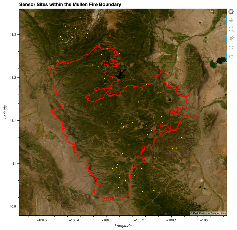
# Combine both
(sensor_plot * boundary_plot).opts(
title='Sensor Sites within the Mullen Fire Boundary',
active_tools=['wheel_zoom']
)
<img src="img/mullen_boundary_and_sites.png" alt="Mullen Wildfire boundary Map including Observation Sites" width="600">